SiteOpt User guide
Introduction
SiteOpt can represent detailed interactions between buildings, local energy production, storage, and the wider grid, allowing planners to explore how different technologies and operating strategies perform over time. By capturing temporal variability such as hourly demand, weather‑driven renewable output, and dynamic electricity prices, SiteOpt helps identify cost‑efficient, low‑carbon solutions for heating, cooling, and electricity supply. Its modular structure also makes it easy to test future scenarios, compare investment options for sustainable district‑level energy planning.
Standard workflow
The standard workflow for SiteOpt usage can be outlined as follows:
- Visualizing the model topology and needed entities in one's own mind or paper
- Starting SiteOpt
- Preparing the input data in form of tabular data (Excel files when using SiteOpt via Spine Toolbox) and CSV files
- Building the model database
- Running optimization and compiling result summary
- Analyzing results
As mentioned on the main page of the documentation, SiteOpt has two user interfaces, Spine Toolbox and the web application. There are small practical differences in the workflow. For example, with the web application, you input the data directly in the user interface, whereas with the Toolbox you prepare input files using Microsoft Excel or other compatible editor.
Visualizing the model topology and needed entities
It is important to understand the way energy systems are abstracted in SiteOpt. Abstraction can be a bit daunting at first but it allows the SiteOpt to model a wider variety of systems instead of limiting to a very restricted set of components. The key idea in the abstraction is that SiteOpt uses only a few simple basic components but parameters are used to modify them so that they can resemble various real life components. Let us now see what these basic components are and what they can be used for. Let us use the following simple example system for this.

In the example you can see different SiteOpt components. Let's see what they mean. Look at the table below.
| Component | Example icon | Description |
|---|---|---|
| Node |  | Node is a place where energy flows meet and demand can take place. This can for example be a consumer point, point of exchange with another subsystem. Often used interchangeably with "block". Indeed, nodes define locations in the model. |
| Renewable unit |  | Renewable units produce either electricity or heat. The production is sent to a specified node. |
| Power-to-heat unit |  | Power-to-heat units produce either heat or cooling using electricity. |
| Connection |  | Connections allow energy transmission. They can be e.g. transmission lines or pipelines. |
| Storage |  | Storages allow energy storage. They can be storages for heat, electricity or cold. |
| Diverting unit |  | unit which produces side streams such as emissions. |
We see that this example system draws electrical energy from the power grid to two loads via connections. The first electrical load node further supplies a radiator unit which supplies a heat load node. The first electrical load node is also connected to a electrical energy storage. The second electrical load node is partly supplied by a PV unit.
Note that in the example system the power grid and loads are also nodes. This is precisely what we mean by using a restricted set of components to model many different real-world items. With these components it is possible to model quite a few different systems. The user should rely on these components when visualizing the model topology. In practise, the recommended steps are:
- Decide the energy vectors which are taken into account: electricity, heat or cooling
- Decide the spatial resolution of demand modelling. For example, does the model "block" refer to a single building, city block or wider area?
- Think about where the whole system is connected to external energy supply, if there is one.
- Think about the grid connections and their detail: is every block connected directly to the external energy supply, is the grid more complex?
Important concepts
To work effectively with the system, it’s important to understand a set of core concepts that define how inputs are organized and how the optimization behaves. The following table lists these core concepts.
| Concept | Description |
|---|---|
| Model | The optimization model which will be created from the user inputs. It holds parameters such as model horizon and time resolution. |
| Block | City block or other location for units. Often used interchangeably with "node". |
| Subunit | Unit of investment for renewable generators, storages and other unit. The user decides the size of subunit. It can be one kW of installed power but also other values are possible. |
| Alternative | A distinct value for certain parameters. For example there can be Base alternative for investment cost and another alternative with lower investment cost. |
| Scenario | Possible realization of all parameters. Composed of one or more alternatives. For example, a scenario may manifest lower investment cost but at the same time lower energy prices. |
| Representative period | A time sample from the defined model horizon which is used to cut down solving time. |
SiteOpt allows scenario analysis. However, scenarios are inputted in a smart way so that you only need to enter the parameters which change between scenarios. There's no need to repeat every parameter value for every scenario. The following picture shows how alternatives are used to help scenario analysis.

In the picture the scenario "My scenario" contains two alternatives in addition to the Base alternative. Alternative 2 has the highest priority, which makes it override all other values. However, it has only been defined for Parameter 1. Alternative 1 overrides the Base value of Parameter 2.
Preparing the input data
The input is mostly given as Microsoft Excel files. Timeseries files are given in comma separated value (CSV) format. When using SiteOpt via Toolbox, you can check the example_data subfolder and copy the files to current_input folder. The input files in the table below are expected to lie in the current_input folder. When using SiteOpt via the Web app, you do not need to manually touch the files. The web application does the file management for you. You can edit data directly in the user interface or upload input files if you have already prepared them.
| Subfolder | Filename | Notes |
|---|---|---|
| nodes/ | nodes.xlsx | node listing and their parameters |
| demand/ | tscr_cooldemand.csv | cooling demand timeseries in SpineOpt format |
| demand/ | tscr_elecdemand.csv | cooling demand timeseries in SpineOpt format |
| demand/ | tscr_heatdemand.csv | heat demand timeseries in SpineOpt format |
| other_units/ | divertingunits.xlsx | special units which create branching flows |
| production/ | pv-input.xlsx | PV and other variable generation unit parameters |
| production/ | hp-input.xlsx | heat pump and chiller unit parameters |
| connections/ | connections_input.xlsx | Connection entity parameters |
| storages/ | storages-input.xlsx | storage unit parameters |
| modelspec.xlsx | model time horizon parameters | |
| scenarios.xlsx | study scenarios definition |
Important Information
It is recommended that you start with the example data set or another dataset provided by an expert user and modify it as needed.
In addition there are two JSON files in the root folder : repr_settings_elexia.json and representative_periods_template.json. The user is normally not expected to touch these.
Not all of the files are expected to containt data. In that case just leave the header row (first row) in the file. In addition to the above mentioned files, the user can also add additional timeseries as CSV files. They can be referenced from the Excel files as explained below.
For detailed instructions on how to fill the data tables, see the section Input data format.
Using SiteOpt via Spine Toolbox
You can use SiteOpt in two ways: via Spine Toolbox or via SiteOpt web application. Here the first method is explained. Refer to the installation section of the documentation to find out how to install SiteOpt for Spine Toolbox.
Introduction to Spine Toolbox
Spine Toolbox is an application, which provides means to define, manage, and execute complex data processing and computation workflows, such as energy system models. It is used as the platform for SiteOpt but it can be used for other purposes. For the interested user, the documentation can be found in Spine Toolbox documentation.
Starting SiteOpt
When using SiteOpt via Spine Toolbox first start the toolbox. Run the commands (using Cmd or Powershell in Windows or shell in Linux)
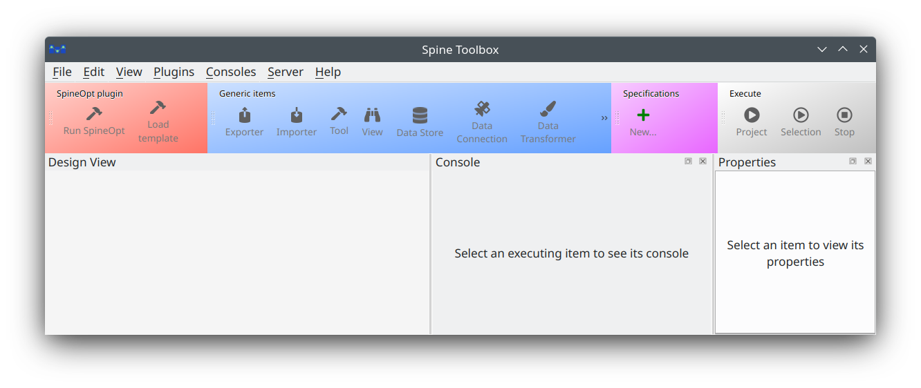
The first time you start the application you will see the main window like this:
Then inside Spine Toolbox:
- Open the project folder where you have downloaded SiteOpt_toolbox: File -> Open project…
- Navigate to the folder where you have downloaded SiteOpt_toolbox
- Press Ok
- If you get a notification to upgrade databases, just upgrade them
- Make sure you also remembered to set Julia settings as described in Installation->Adjust toolbox settings
Building the database for optimization
The SiteOpt inputs need to be translated to a format which is understood by the optimization model. This should be done each time you change the inputs (i.e. the Excel files described above or the time series CSV files).
- Close the input Excel files
- Observe the Design view window in the toolbox
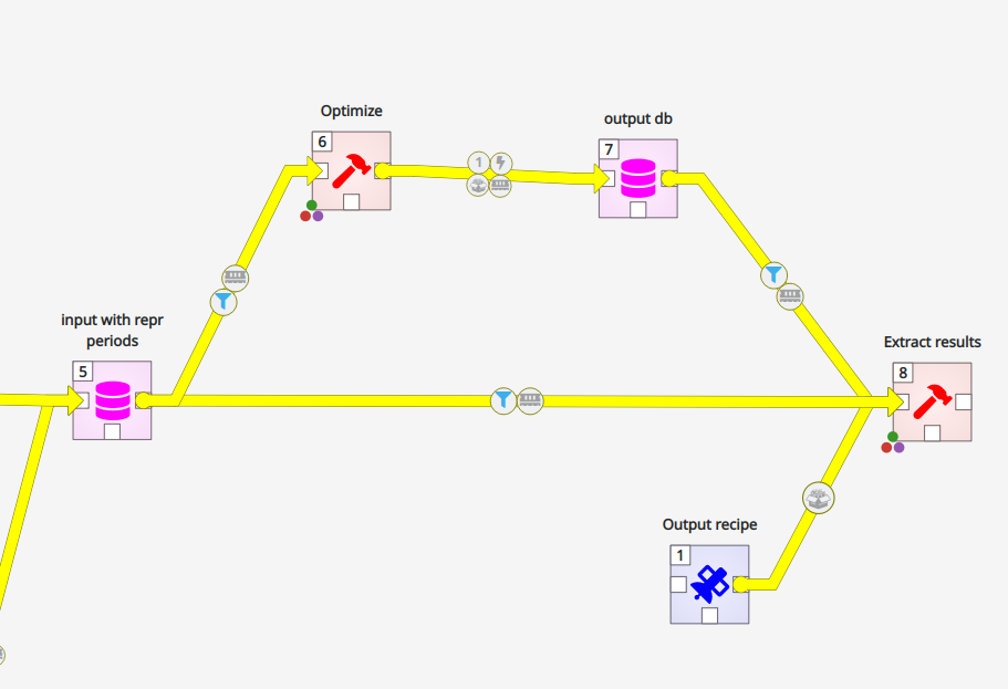
- Using left mouse button held, select everything to the left of the pink ”Input data” box (see figure). It does not matter if you select the blue components or not.
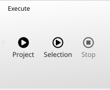
- In the top toolbox press Execute Selection
- Wait until all the hammer tools have a green check mark
- Red cross in tool icon means an error
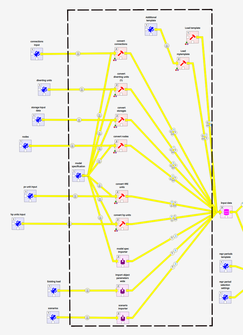
Building the database can take several minutes. When all the components within your selection turn green, the database has been finished.
Running representative periods selection
Representative periods are a way to simplify long‑term energy system studies without losing the big picture. Instead of simulating every hour of an entire year — which would be extremely heavy to compute — the year is broken into a small number of “typical” days that capture the main patterns in demand and renewable generation. Think of it like choosing a few key scenes from a movie that still let you understand the whole story. In SiteOpt, you can either use representative periods or not. If you decide to use them, select and run (press Execute selection) the Select repr periods component right of the Input data. When the Select repr periods component has turned green, the selection has been finished.
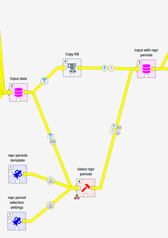
Select repr periods component right of the Input data by using left mouse button.
Running optimization
Optimization of the model can be started by selecting the Optimize tool in Toolbox and clicking "Execute selection" in the toolbar. Before this, click the data path coming to the Optimize tool from the left. In the link properties window you can now see the scenarios which are selected for optimization. Select the ones you want. If the properties window is not visible, select View menu -> Dock widgets->Link properties.
Optimize component using left mouse button.
Running the optimization can take anything from a few minutes to tens of minutes. Reducing the number of nodes and optimized units as well as increasing time resolution can reduce the running time.
You can also select the Extract results component, which builds an Excel summary of the results, at the same time with optimization or after it. The Excel summary can be accessed by right-clicking the Extract results component and selecting "Open results directory". There the results have been arranged according to the run time.
Using SiteOpt via the SiteOpt web app
The SiteOpt web app provides a more intuitive user interface for SiteOpt. It is used via a web browser. It uses the same input data as the basic SiteOpt but the data is entered via its interface (you can also import Excel files if you have them ready) The installation steps have been explained in the installation section of the documentation.
Basics
You start SiteOpt web app by first starting Docker Desktop, start command prompt in the folder where you have installed SiteOpt web app, and then run the command
and point your browser to http://localhost/. There is also a "developer version" of the tool. The starting procedure is slightly different for this. Refer to the web app installation instructions.
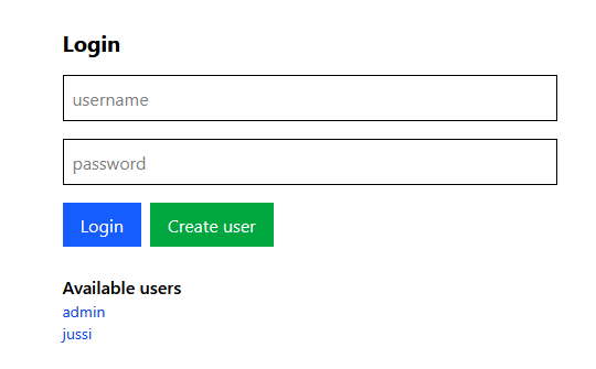
You first enter a login page as shown below. Choose a user name and password and click Create user. Later you just click Login. There can be many users and each user has her own datasets. Logging out is possible from the upper right corner of the main window.
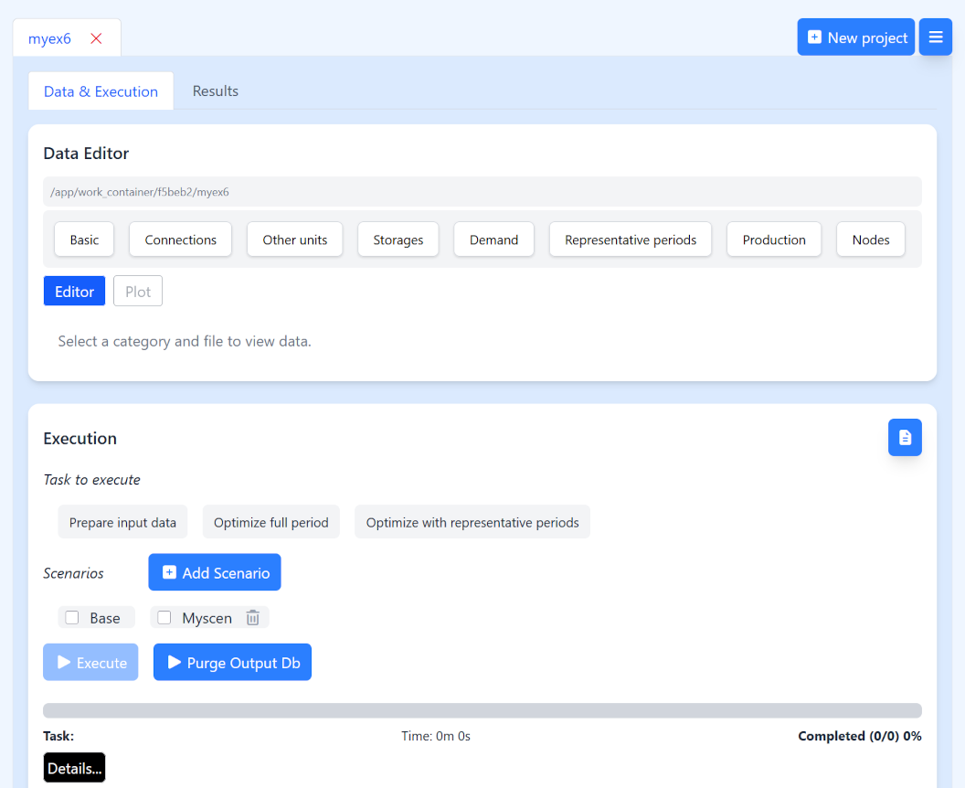
In the figure below you can see the application window. It consists of two tabs: Data & execution and results. The Data & execution tab is for editing input data and running the tool. The results tab then presents the results as graphs. Also, on the upper level there is the project tab. Each project has its own data and results tabs. This will be explained next.
Creating projects
On top of the window, you can see that there is a tab called "myex6". This is the project name. You can have many projects, each with their own set of input data and results. You can create a new project by pressing the New project button. The program asks which dataset you want to copy as basis. The options are:
- Dokken dataset describing Elexia Dokken pilot;
- Dokken light dataset describing Elexia Dokken pilot (a more compact dataset resulting in a smaller model and shorter run times)
- small example dataset useful for learning
Select the dataset and project name and press "Ok". The project appears as a new tab. You can remove project tab from the window by pressing the X button
Important Information
When running the development version you must have access to the Git repository holding the Dokken datasets to use them. If you use the production version, the datasets are already included in your software.
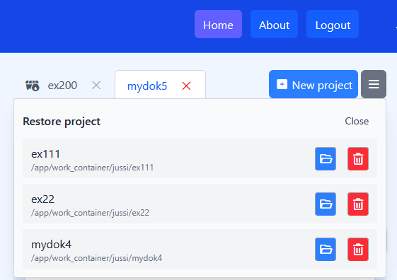
If you click the hamburger icon in the top right corner of the window, you can see all your saved projects. This includes the ones which you previously closed. There you can delete projects permanently or reopen them.
Editing data
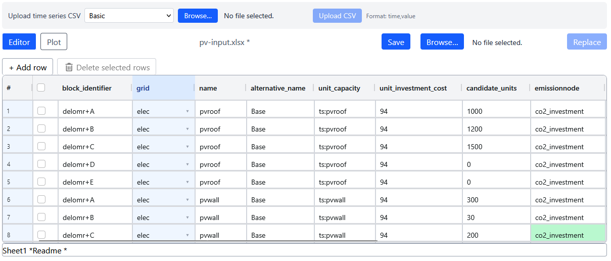
The main window of the SiteOpt web app with normally has the data and execution tab open. This tab contains two panes: Data editor and Execution. Data editor lets you view and edit the input data files in the project. These are precisely the files described above. For example, to edit VRE production units, click Production button and select "pv-input.xlsx". The Excel file opens in the editor and you can make changes. You can:
- edit individual cells
- copy and paste values to/from individual cells
- delete a row by ticking the box in front of the row and pressing
Delete selected - add new rows to the bottom by pressing
Add row - replace the whole file by a file on your computer by pressing first
Browse, selecting a file of the same name, pressOpenand thenReplace - upload a time series file in CSV format by first selecting the folder it goes to from a dropdown menu. The folder should be the same one where it is referenced.
Upload CSVadds the file to the project. - change sheets in the file from the tabs below the data table. This applied only to files which have multiple sheets, such as "modelspec.xlsx".
- save the edited data by pressing
Save(or CTRL-S) - discard the edits by selecting some other file and clicking
discardwhen prompted.
You will notice that some cells accepts text values, others numeric values (or timeseries references preceeded by "ts:"), and still others a selection of predefined values. If you make a reference to a time series, there is a button which allows you to upload the corresponding CSV file. A wrong type of data causes the cell to be highlighted. You will also see an exclamation mark next to the file name in the data editor.
Refer to the guidelines in the “Preparing input data” section for the required data‑input format.
Running the model
Execution tab lists tasks which you can perform ("Task to execute"). These include:
- Prepare input data: SiteOpt inputs need to be translated to a format which is understood by the optimization model. This task builds the input database.
- Optimize full period: performs optimization using the full model horizon defined in modelspec.xslx. Especially for bigger models this can take 10–20 minutes or even more.
- Optimize full period: select samples from the full model horizon defined in modelspec.xslx and then perform optimization. This is normally the faster but less accurate option.
You first select a task and then press Execute. You have to prepare input data before running optimization. You also have to prepare input data each time you make changes to the input data files. Before optimization you also have to select one or more scenarios. During execution the progress bar tracks the execution stage.
Purge Output Db clears the results database to remove clutter and save space.
Important Information
When Optimizing with full period the solution can be slow. However it is safe to use this option with the example model and other small models where there are not many nodes and the time horizon is short.
Important Information
Remember to update input database (prepare input data) each time you make changes to the input data files.
Viewing results
On top of the page you can switch to Results dashboard tab. Note that you first have to have some calculated results. Otherwise the tab shows message "Run the model to generate result files." The results are organized by scenario and optimization run time. During each optimization run, results summary is produced for all the results which have been stored in the output database. This is why you may sometimes see quite many scenarios in the figures. You can clear the output database by pressing Purge Output Db on the Data & execution tab.
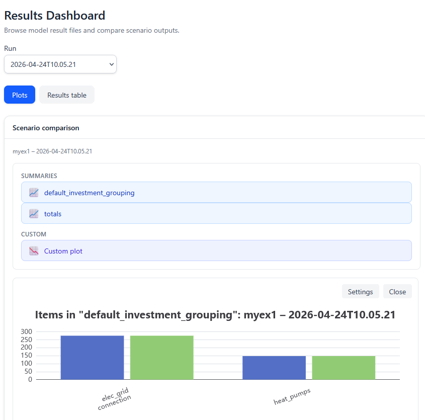
The figure above shows a screenshot of the results dashboard. There is first a dropdown box for selecting the optimization run. In scenario comparison window you see the project name and the selected run time. In "Summaries" you can select three different types of figures:
- Totals summary (top-level key performance metrics)
- Default investment grouping: total optimized investment into pre-defined entity categories
- Custom plot where you can select the categories and scenarios included.
You can turn on and off the first two figures by clicking their labels in the "Summaries" selection. Clicking the custom plot label takes you to a window where you can select the categories and scenarios included.
The pre-defined entity categories include as categories:
- renewable energy (VRE) units (currently not broken down)
- heat pump and chiller units
- connections of different grids
- storages in different grids
The top-level key performance metrics include:
- total costs of the defined system
- variable costs of the defined system (includes connection flow costs and emissions costs)
- supply chain CO2 emissions originating from plant investments
- your project settings may have other metrics included, such as emissions related to purchased electricity Notice that the metrics are calculated for the model period. In other words, if you have set model_start and model_end parameters in modelspec.xlsx so that the model spans one year, then the values are calculated for one year period. Using represenative periods does not change this, although the result will be approximated.
In the results view you cannot view detailed results such as decision variable values at specific time point. However, advanced users can modify the plot figure contents by editing output_recipe.json file in the project data folder.
Input data format reference
In the following we will go through each of the input files and show how to fill them.
The nodes table
In nodes.xlsx each row represents one node. However, you can give several alternative parameter values for a node, and in this case each alternative makes one row. Also, you have to define the different grids for each node. For example if cooling demand exists in a node, you have to add a row where grid is "cool".
| Column | Required | Description |
|---|---|---|
| node | x | Node name or block name |
| grid | x | The type of energy or material transferred: "elec", "heat" or "cool" |
| alternative_name | x | The alternative which the given values refer to (normally "Base"). Can be left empty if no values are given. |
| free_node | Can define the node as free node. Normally balance accounting is forced in a node, so that energy is not created or does not disappear. An "X" disables the balance accounting. | |
| demand | Demand of energy or material in the node. If constant, just input a number. If it is a timeseries, follow the notation given in section "Entering data". | |
| representative_node | An "X" takes the demand timeseries into account when choosing representative periods |
Node names should be unique. However, you can use the same name in different grids. Normally nodes keep track of energy balance. However, if one declares free node then no such condition is enforced. You should use this option for nodes which act as an interface to the external world, e.g. point of common coupling.
If you wish to define values (e.g. demand) for different alternatives, add a separate row for each node and alternative. Notice that demand time series can also be inputted as shown in the next section.
The table below shows an example nodes table. There we define two electrical nodes where node n1 is an electrical bus with no demand. n2 has demand in timeseries format, and file ts_demand2.csv should be present in the nodes folder. This timeseries is used when selecting representative periods. In the alternative newalt the demand of node n2 has been changed to another timeseries.
| node | grid | alternative_name | free_node | demand | representative_node |
|---|---|---|---|---|---|
| n1 | elec | Base | |||
| n2 | elec | Base | ts:demand2 | -X- | |
| n2 | elec | newalt | ts:demand2b | -X- |
Demand data
Demand data for three grids (electricity, heating and cooling) can be given in cross-tabulated CSV files. These are:
- tscr_cooldemand.csv for cooling demand timeseries
- tscr_elecdemand.csv for electricity demand timeseries
- tscr_heatdemand.csv for heat demand timeseries
The format of these files is the following:
| Column header | Required | Description |
|---|---|---|
| Objectclass | x | "node" without parentheses |
| Parameter_name | x | "demand" without parentheses |
| alternative | x | The alternative which the given values refer to (normally "Base" without parentheses) |
| time | x | Timestamp in ISO8601 format YYYY-MM-DDTHH:mm:SS |
| n_1_elec | Any following columns should have header name of the node in SpineOpt format. It should be preceeded by "n_" then have the block name followed by the grid name e.g. "_elec". The column then contains the actual values. |
It is probably obvious to the user that these files are not meant to be populated manually but using spreadsheet software or other software for processing time series data. Note that you don't need to input demand data via these files. You can also specify timeseries in the nodes input table. In that case you need a separate file for each node and grid.
Production units table
In pv_units.xlsx the user defines renewable generation units such as PV units and wind turbines or solar collectors.
| Column | Required | Description |
|---|---|---|
| block_identifier | x | Node name |
| grid | x | The type of energy produced: "elec", "heat" or "cool" (without quotation marks) |
| name | x | The name of the unit, which should be different if there are different units in the same block. |
| alternative_name | x | The alternative which the given values refer to (normally "Base" without quotation marks) |
| unit_capacity | x | The capacity of one subunit (e.g. kilowatts). Normally here one enters the time series for the capacity factor of the unit. |
| unit_investment_cost | The investment cost of one subunit as annualized cost (e.g. €/kW/year if subunit is 1 kW). | |
| candidate_units | The maximum number of subunits which can be built. | |
| representative_unit | An "X" indicates that the capacity factor of this unit will be used when selecting the representative periods for optimization. |
There are also data related to the supply chain carbon dioxide emissions of the production units:
| Column | Required | Description |
|---|---|---|
| emissionnode | You are expected to enter the name of a free node which collects the emissions | |
| investment_emission | The hourly carbon dioxide emission arising from one subunit (e.g. kg/hour) | |
| emission_cost | The cost of these carbon dioxide emissions (e.g. €/kg) |
The emission nodes currently do not belong to any grid, so leave the grid column empty when defining them in the nodes table.
If you wish to define parameter values for different alternatives, add a separate row for each unit and alternative. Below you can see an example of what the renewable production units table can look like. In this example, the unit is producting electricity and the capacity factor (production profile) is given as time series (in a CSV file). The cost of one subunit is 100 monetary units per year and the maximum number of subunits is 40 (10 subunits in alternative newalt).
| block_identifier | grid | name | alternative_name | unit_capacity | unit_investment_cost | candidate_units | representative_unit |
|---|---|---|---|---|---|---|---|
| b1 | elec | basic_pv | Base | ts:pv | 100 | 40 | |
| b1 | elec | basic_pv | newalt | ts:pv | 100 | 10 |
Important Information
In SiteOpt the user should decide the units of measurement. For example the user for power can be kW or MW. Currency unit can be € or Norwegian krone. Any any case, units should be used consistently.
Heat pumps and chiller units table
In hp_units.xlsx the user defines heat pumps and chillers. Unlike renewable generation units (defined in pv_units.xlsx) these technologies require electricity to operate.
| Column | Required | Description |
|---|---|---|
| block_identifier | x | City block name |
| type | x | The type of energy produced: "heat" or "cool" without quotation marks |
| alternative_name | x | The alternative which the given values refer to (normally "Base" without quotation marks) |
| sourcegrid | The grid where energy is drawn from for the unit. It can be left empty if you wish to disregard the source (e.g. ambient air). | |
| unit_capacity | x | The capacity of one subunit (e.g. kilowatts). Normally here one enters the time series for the capacity factor of the unit. |
| unit_investment_cost | The investment cost of one subunit as annualized cost (e.g. €/kW/year if subunit is 1 kW). | |
| cop_profile | x | The coefficient of performance (COP) factor (unitless) |
| candidate_units | The maximum number of subunits which can be built. |
In addition there are also data related to the supply chain carbon dioxide emissions of the production units. They are defined the same way as for renewable production units.
Group potentials table
Normally, investments into different VRE units are independent. However, if for example they share the same area, potentials for certain groups of units can be defined. In group_potential.xlsx the user defines aggregated renewable unit investment potentials for PV units and wind turbines or solar collectors.
| Column | Required | Description |
|---|---|---|
| block_identifier | x | Node name |
| grid | x | The type of energy produced: "elec", "heat" or "cool" (without quotation marks) |
| name | x | The name of the unit, which can be the same if the unit exists in many blocks |
| alternative_name | x | The alternative which the given values refer to (normally "Base" without quotation marks) |
| group | x | The name of the group for which an investment constraint is given. Can be selected freely. |
| candidate_units | x | The quantity of total invested subunits allotted to this group. |
For example, if you wish to create an aggregated investment constraint which pertains to two different units, add two lines to this file. Input the unit blocks, grids and names as in pv_input.xslx. Think of a descriptive and unique name for this constraint and put it into the groupcolumn on both lines. On one (not both) of the lines in candidate_units columns, write the maximum number of subunits which can be invested.
Connections table
In SiteOpt and SpineOpt connections are entities which can transfer energy and material from one node to another. These include power lines and pipelines. However, as SiteOpt works in an abstract level, it does not require that you specify what type of real infrastructure the connection represents. Instead you enter parameters which determine how these connection behave.
In connections_input.xlsx each row represents one connection entity. The header row shows what is expected on each column. The columns are as follows:
| Column | Required | Description |
|---|---|---|
| node1 | x | The originating city block of the connection. |
| node2 | x | The destination city block of the connection. |
| grid | x | The type of energy transferred: "elec" (electricity), "heat" (heating) or "cool" (cooling) . |
| alternative_name | x | The alternative which the given values refer to (normally "Base"). |
| connection_flow_cost | The unit cost of energy or material transfer, e.g. €/kWh. | |
| connection_flow_cost.mul | Multiplier for the unit cost of energy or material transfer, e.g. to convert between units between the model and input data. | |
| connection_flow_cost_reverse | The unit cost of energy or material transfer in reverse direction (i.e. from node 2 to node 1). | |
| connection_flow_cost_reverse.mul | Multiplier for the unit cost of energy or material transfer in reverse direction | |
| connection_capacity | X | Capacity of one subunit of connections. Total capacity if there are no candidate connections. |
| connection_investment_cost | Annual investment cost of one subunit of connections. Can be empty if investments are not targeted. | |
| candidate_connections | Maximum number of subunits of connections which can be invested | |
| efficiency | Transfer efficiency (e.g. 0.95 meaning 95 %) dictates how much of the transfed quantity reaches the destination and how much is lost. |
It is important that you keep in mind the choices for capacity (e.g. connection_capacity) and energy variables (e.g. connection_flow_cost).
The following shows an example connections table. For example node A1 is connected to node B3 in electricity grid. It is a connection which can be dimensioned by the tool, with maximum 3 subunits, each having a capacity of 1 power unit.
| node1 | node2 | grid | alternative_name | connection_flow_cost | connection_flow_cost.mul | connection_flow_cost_reverse | connection_flow_cost_reverse.mul | connection_capacity | connection_investment_cost | candidate_connections | efficiency |
|---|---|---|---|---|---|---|---|---|---|---|---|
| A1 | B3 | elec | Base | 0.12 | 0.14 | 1.0 | 120 | 3 | 0.95 | ||
| C1 | D1 | heat | Base | 0.05 | 0.06 | 15.0 | 0.90 | ||||
| E1 | F2 | cool | Base | 0.08 | 0.09 | 1.0 | 90 | 7 | 0.92 |
Storages table
In storages-input.xlsx the user defines electricity, heat and cold storages. The input table format is shown below.
| Column | Required | Description |
|---|---|---|
| block_identifier | x | Block name (node name). |
| type | x | The type of energy produced: "heat" or "cool" |
| alternative_name | x | The alternative which the given values refer to (normally "Base") |
| capacity | x | Storage capacity (e.g. kWh) of one storage subunit |
| max_charging | x | Charging capacity (e.g. kW) of one storage subunit |
| max_discharging | x | Discharging capacity (e.g. kW) of one storage subunit |
| demand | Possible energy demand drawn directly from the storage | |
| unit_investment_cost | x | Annualized investment cost of the charger/discharger (per subunit) |
| storage_investment_cost | x | Annualized investment cost of storage section (per subunit) |
| candidate_units | x | Maximum number of charger/discharger subunits |
| candidate_storages | x | Maximum number of storage section subunits |
| storage_investment_variable_type | x | Decides whether fractional subunits can be built. |
The storage table is more complex than the other tables because the power conversion section (charger and discharger) is defined separately from the actual storage. Thus an investment cost is given both from the storage capacity and charger power. These are given for one subunit on an annual basis as usual. The maximum number of subunits is be given both for the storage section and charger section. Normally it is convenient to define one subunit as kW or MW for charger and kWh or MWh for the storage section but they may also be defined e.g. according to certain battery model if it is convenient for the user.
Also the storage table contains the columns related to investment emissions. See the section about production units table for instructions on how to fill them.
Diverting units table
Diverting units create side streams from energy or material flow. They are e.g. used for internal emission accounting purposes of the optimization model. The input table format is shown below.
| Column | Required | Description |
|---|---|---|
| name | x | Name of the unit |
| inputgrid | x | Name of the grid where the input comes from |
| inputnode | x | Name of the node within the input grid |
| outputgrid | Name of the grid where the main output goes to | |
| outputnode | x | Name of the node within the output grid where the main output goes to |
| divertinggrid | x | Name of the grid where the side stream goes to |
| divertingnode | x | NName of the node where the side stream goes to |
| alternative_name | x | The alternative to which the parameters apply to |
| diversionfactor | x | The magnitude of the side stream compared to main input |
| vom_cost | x | The variable cost arising from the side stream |
Modelspec table
The modelspec.xlsx file contains five sheets but only two of them are normally needed by the user. params_1d_datetime contain the following data about the model time horizon:
| Column | Required | Description |
|---|---|---|
| objectclass | x | enter text model |
| object | x | enter text mymodel |
| parameter_name | x | either model_start or model_end |
| alternative_name | x | The alternative which the given values refer to (normally Base) |
| parameter_value | x | The model start or end time in YYYY-MM-DDTHH:mm:ss format |
In other words, here you adjust which parts of the given time series are used for optimization. As suggested by the sheet name, the values are given as datetimes. The longer the model horizon, the more reliable the results will be. Notice that the time series which you use must cover the model horizon.
params_1d_durations sheet contain data about the time resolution used by optimization. Normally it contains two rows. One of the rows determines the time resolution used in the day-to-day optimization of the system. The other defines how often investments can be made. Presently SiteOpt supports only a single investment for each entity, so the time resolution for investments should be longer than the model horizon.
| Column | Required | Description |
|---|---|---|
| objectclass | x | enter text temporal_block |
| object | x | enter text myblock or myinvestmentblock |
| parameter_name | x | enter text resolution |
| lternative_name | x | The alternative which the given values refer to (normally Base) |
| parameter_value | x | The model time resolution (normally 1 hour 1 hfor myblock and 1 year 1 Y for myinvestmentblock |
It is suggested that you keep the values as 1 hfor myblock but you may increase the value to several hours to speed up computation. For myinvestmentblock you can use e.g. 1 Y (keep it longer than the model horizon).
Scenarios table
The scenarios.xlsx file contains three sheets. The scenario sheet just lists the different scenario names in the first column (first row just is header row). Likewise the alternative sheet lists different alternatives in the first column, where the first row is header row. scenario_alternative sheet is more complex and has two kind of entries. On this sheet, the first column (A) is reserved for scenario names and two next columns (B-C) for alternative names. When two columns (A and B) are filled, this has the meaning that an alternative belongs to a scenario. When three columns (A, B and C) are filled, this has the meaning of defining the order of alternatives. In this case the alternative written in column C has higher precedence and alternative written in column B. If There are more than 2 alternatives in any scenario, more rows should be used to define the order of the alternatives.
The following picture shows an example.

Highpricealternative overrides the Base alternative in Myscen scenario.
Entering data
You will need different types of data for different parameter indices and values. The following datatypes can be entered in the input tables.
| Type | Example | Notes |
|---|---|---|
| text | n_7_elec | use letters, numbers, dashes, plus-signs and underscores |
| number | 7.1 | scientific notation such as 1.0e3 is also allowed |
| Datetime | 2025-12-31T13:00:00 | Format YYYY-MM-DDTHH:mm:ss |
| Duration | 3h | Represents a time duration. The unit can be either Y (for year), M (for month), D (for day), h (for hour), m (for minute), or s (for second). |
| timeseries | ts:elec7 | always begin with ts: |
For datetimes such as time stamps the recommended format is ISO8601 (e.g. 2020-03-01T01:00). In case of timeseries, the actual timeseries data should be placed in a CSV file (text file where column are separated by commas) in the input data folder (same folder as the referencing Excel file). If you use the SiteOpt web application, there is a button which allows you to select a CSV file on your computer and upload it. The file should have two columns which have column titles "time" and "value". File name should have the format ts_ + time series name + .csv. For example if you write ts:elec7 in the input data table, file name ts_elec7.csv is expected. Note that SiteOpt does not make daylight saving time adjustments.

For durations the data should be entered in format xU where x is an integer and U is either Y (for year), M (for month), D (for day), h (for hour), m (for minute), or s (for second). For example "60m".